Examples
Some examples on how to use certain layers.
Fitting backbone using reduced protein model.
First we read the pdb file using FullAtomModel.PDB2CoordsUnordered:
 Next we plot aligned structures that we saved during optimization:
#Reading pdb file
p2c = FullAtomModel.PDB2CoordsUnordered()
coords_dst, chain_names, res_names_dst, res_nums_dst, atom_names_dst, num_atoms_dst = p2c(["FullAtomModel/f4TQ1_B.pdb"])
#Making a mask on CA, C, N atoms
is0C = torch.eq(atom_names_dst[:,:,0], 67).squeeze()
is1A = torch.eq(atom_names_dst[:,:,1], 65).squeeze()
is20 = torch.eq(atom_names_dst[:,:,2], 0).squeeze()
is0N = torch.eq(atom_names_dst[:,:,0], 78).squeeze()
is10 = torch.eq(atom_names_dst[:,:,1], 0).squeeze()
isCA = is0C*is1A*is20
isC = is0C*is10
isN = is0N*is10
isSelected = torch.ge(isCA + isC + isN, 1)
num_backbone_atoms = int(isSelected.sum())
#Resizing coordinates array for convenience
N = int(num_atoms_dst[0].item())
coords_dst.resize_(1, N, 3)

backbone_x = torch.masked_select(coords_dst[0,:,0], isSelected)[:num_backbone_atoms]
backbone_y = torch.masked_select(coords_dst[0,:,1], isSelected)[:num_backbone_atoms]
backbone_z = torch.masked_select(coords_dst[0,:,2], isSelected)[:num_backbone_atoms]
backbone_coords = torch.stack([backbone_x, backbone_y, backbone_z], dim=1).resize_(1, num_backbone_atoms*3).contiguous()
#Setting conformation to alpha-helix
num_aa = torch.zeros(1, dtype=torch.int, device='cuda').fill_( int(num_backbone_atoms/3) )
num_atoms = torch.zeros(1, dtype=torch.int, device='cuda').fill_( int(num_backbone_atoms) )
angles = torch.zeros(1, 3, int(num_backbone_atoms/3), dtype=torch.float, device='cuda').normal_().requires_grad_()

a2b = ReducedModel.Angles2Backbone()
rmsd = RMSD.Coords2RMSD()

optimizer = optim.Adam([angles], lr = 0.05)
loss_data = []
g_src = []
g_dst = []

#Coords transforms
c2c = FullAtomModel.Coords2Center()
translate = FullAtomModel.CoordsTranslate()
rotate = FullAtomModel.CoordsRotate()

#Rotating for visualization convenience
with torch.no_grad():
	backbone_coords = rotate(backbone_coords, torch.tensor([[[0, 1, 0], [-1, 0, 0], [0, 0, 1]]], dtype=torch.float, device='cuda'), num_atoms)
for epoch in range(300):
	optimizer.zero_grad()
	coords_src = a2b(angles, num_aa)
	L = rmsd(coords_src, backbone_coords, num_atoms)
	L.backward()
	optimizer.step()

	loss_data.append(L.item())
	#Obtaining aligned structures
	with torch.no_grad():
		center_src = c2c(coords_src, num_atoms)
		center_dst = c2c(backbone_coords, num_atoms)
		c_src = translate(coords_src, -center_src, num_atoms)
		c_dst = translate(backbone_coords, -center_dst, num_atoms)
		rc_src = rotate(c_src, rmsd.UT.transpose(1,2).contiguous(), num_atoms)

		rc_src = rc_src.resize( int(rc_src.size(1)/3), 3).cpu().numpy()
		c_dst = c_dst.resize( int(c_dst.size(1)/3), 3).cpu().numpy()

		g_src.append(rc_src)
		g_dst.append(c_dst)
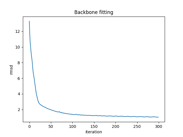
fig = plt.figure()
plt.title("Backbone fitting")
plt.plot(loss_data)
plt.xlabel("iteration")
plt.ylabel("rmsd")
plt.savefig("ExampleFitBackboneTrace.png")
#Plotting result
fig = plt.figure()
plt.title("Reduced model")
ax = p3.Axes3D(fig)
sx, sy, sz = g_src[0][:,0], g_src[0][:,1], g_src[0][:,2]
rx, ry, rz = g_dst[0][:,0], g_dst[0][:,1], g_dst[0][:,2]
line_src, = ax.plot(sx, sy, sz, 'b-', label = 'pred')
line_dst, = ax.plot(rx, ry, rz, 'r.-', label = 'target')

def update_plot(i):
    sx, sy, sz = g_src[i][:,0], g_src[i][:,1], g_src[i][:,2]
    rx, ry, rz = g_dst[i][:,0], g_dst[i][:,1], g_dst[i][:,2]
    line_src.set_data(sx, sy)
    line_src.set_3d_properties(sz)

    line_dst.set_data(rx, ry)
    line_dst.set_3d_properties(rz)

    return line_src, line_dst

anim = animation.FuncAnimation(fig, update_plot,
                                    frames=300, interval=20, blit=True)
ax.legend()
anim.save("ExampleFitBackboneResult.gif", dpi=80, writer='imagemagick')