ReducedModel
This module contains implementation of angles to coordinates conversion for reduced protein models.
This layer converts the dihedral angles describing the backbone conformation of a protein to the coordinates of the backbone atoms.
During the forward pass, we save the products of transformation matrices for each atom: $$A_i = B_0 B_1 \cdots B_i$$ Notice that atom $3j$ is always N, atom $3j + 1$ is always CA, and atom $3j+2$ is always C. Thus transformation matrices $B_{3j+1}$ and $B_{3j+2}$ depend on the angles $\phi_j$ and $\psi_j$, correspondingly.
During the backward pass, we first compute the gradient of $\mathbf{x}_i$, the position of atom $i$, with respect to each "$\phi$" and "$\psi$" angle: $$ \frac{\partial \mathbf{x}_i}{\partial \phi_j} = B_0 B_1 \cdots \frac{\partial B_{3j+1}}{\partial \phi_j} \cdots B_i \mathbf{x}_0 $$ $$ \frac{\partial \mathbf{x}_i}{\partial \psi_j} = B_0 B_1 \cdots \frac{\partial B_{3j+2}}{\partial \psi_j} \cdots B_i \mathbf{x}_0 $$ We can rewrite these expressions using the matrices $A$ that we saved during the forward pass: $$ \frac{\partial \mathbf{x}_i}{\partial \phi_j} = A_{3j} \frac{\partial B_{3j+1}}{\partial \phi_j} A_{3j+1}^{-1} A_{i} \mathbf{x}_0 $$ $$ \frac{\partial \mathbf{x}_i}{\partial \psi_j} = A_{3j+1} \frac{\partial B_{3j+2}}{\partial \psi_j} A_{3j+2}^{-1} A_{i} \mathbf{x}_0 $$ Both the $A$ and $B$ matrices have the form: $$ T = \begin{bmatrix} R & \mathbf{x} \\ 0 & 1 \end{bmatrix} $$ and their inverses can be computed as follows: $$ T^{-1} = \begin{bmatrix} R^{T} & -R^{T}\mathbf{x} \\ 0 & 1 \end{bmatrix} $$ This allows us to compute all derivatives simultaneously on GPU. To compute the derivatives of the layer output $L$ with respect to the input angles, we just have to calculate the following sums: $$\sum_i \frac{\partial L}{\partial \mathbf{x}_i}\cdot \frac{\partial \mathbf{x}_i}{\partial \phi_j}$$ and $$\sum_i \frac{\partial L}{\partial \mathbf{x}_i}\cdot \frac{\partial \mathbf{x}_i}{\partial \psi_j}$$
from TorchProteinLibrary import ReducedModel
a2b = ReducedModel.Angles2Backbone()
angles = torch.randn(1, 3, 3, dtype=torch.float, device='cuda')
num_aa = torch.tensor([3], dtype=torch.int, device='cuda')
coords = a2b(angles, num_aa)
Implementation
The position of the $i$-th atom in the chain is obtained by: $$\mathbf{x}_i = B_0 B_1 \cdots B_i \mathbf{x}_0$$ where $\mathbf{x}_0$ is the position of the atom in the original reference frame and $B_i$ are transformation matrices parametrized by dihedral angles: $$B(\alpha, \beta, d) = \begin{bmatrix} \cos(\beta) & \sin(\alpha)\sin(\beta) & \cos(\alpha)\sin(\beta) & d\cos(\beta) \\ 0 & \cos(\alpha) & -\sin(\alpha) & 0 \\ -\sin(\beta) & \sin(\alpha)\cos(\beta) & \cos(\alpha)\cos(\beta) & -d\sin(\beta) \\ 0 & 0 & 0 & 1 \end{bmatrix}$$ The transformations are defined as follows:-
$C$-$N$ peptide bond of residue $j-1$:
Index: $i = 3j$
Transformation: $ B_i = B(\omega_{j-1}, \pi - 2.1186, 1.330)$ -
$N$-$C_{\alpha}$ bond of residue $j$:
Index: $i = 3j + 1$
Transformation: $ B_i = B(\phi_{j}, \pi - 1.9391, 1.460)$ -
$C_{\alpha}$-$C$ bond of residue $j$:
Index: $i = 3j + 2$
Transformation: $ B_i = B(\psi_{j}, \pi - 2.061, 1.525)$
During the forward pass, we save the products of transformation matrices for each atom: $$A_i = B_0 B_1 \cdots B_i$$ Notice that atom $3j$ is always N, atom $3j + 1$ is always CA, and atom $3j+2$ is always C. Thus transformation matrices $B_{3j+1}$ and $B_{3j+2}$ depend on the angles $\phi_j$ and $\psi_j$, correspondingly.
During the backward pass, we first compute the gradient of $\mathbf{x}_i$, the position of atom $i$, with respect to each "$\phi$" and "$\psi$" angle: $$ \frac{\partial \mathbf{x}_i}{\partial \phi_j} = B_0 B_1 \cdots \frac{\partial B_{3j+1}}{\partial \phi_j} \cdots B_i \mathbf{x}_0 $$ $$ \frac{\partial \mathbf{x}_i}{\partial \psi_j} = B_0 B_1 \cdots \frac{\partial B_{3j+2}}{\partial \psi_j} \cdots B_i \mathbf{x}_0 $$ We can rewrite these expressions using the matrices $A$ that we saved during the forward pass: $$ \frac{\partial \mathbf{x}_i}{\partial \phi_j} = A_{3j} \frac{\partial B_{3j+1}}{\partial \phi_j} A_{3j+1}^{-1} A_{i} \mathbf{x}_0 $$ $$ \frac{\partial \mathbf{x}_i}{\partial \psi_j} = A_{3j+1} \frac{\partial B_{3j+2}}{\partial \psi_j} A_{3j+2}^{-1} A_{i} \mathbf{x}_0 $$ Both the $A$ and $B$ matrices have the form: $$ T = \begin{bmatrix} R & \mathbf{x} \\ 0 & 1 \end{bmatrix} $$ and their inverses can be computed as follows: $$ T^{-1} = \begin{bmatrix} R^{T} & -R^{T}\mathbf{x} \\ 0 & 1 \end{bmatrix} $$ This allows us to compute all derivatives simultaneously on GPU. To compute the derivatives of the layer output $L$ with respect to the input angles, we just have to calculate the following sums: $$\sum_i \frac{\partial L}{\partial \mathbf{x}_i}\cdot \frac{\partial \mathbf{x}_i}{\partial \phi_j}$$ and $$\sum_i \frac{\partial L}{\partial \mathbf{x}_i}\cdot \frac{\partial \mathbf{x}_i}{\partial \psi_j}$$
Input/Output
Example
import torch
from TorchProteinLibrary import ReducedModel
import numpy as np
import matplotlib.pylab as plt
import mpl_toolkits.mplot3d.axes3d as p3
if __name__=='__main__':
a2b = ReducedModel.Angles2Backbone()
#Setting conformation to alpha-helix
N = 20
num_aa = torch.zeros(1, dtype=torch.int, device='cuda').fill_(N)
angles = torch.zeros(1, 3, N, dtype=torch.float, device='cuda')
angles[:,0,:] = -1.047 # phi = -60 degrees
angles[:,1,:] = -0.698 # psi = -40 degrees
angles[:,2,:] = np.pi # omega = 180 degrees
#Converting angles to coordinates
coords = a2b(angles, num_aa)
num_atoms = num_aa*3
#Resizing coordinates array for convenience (to match selection mask)
N = int(num_atoms.data[0])
coords.resize_(1, N, 3)
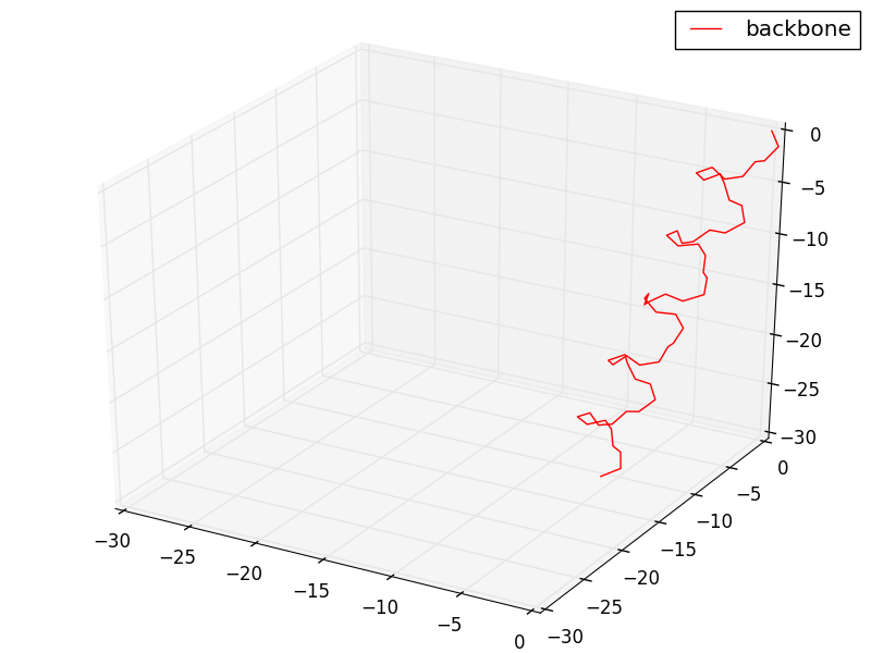
#Plotting backbone
sx, sy, sz = coords[0,:,0].cpu().numpy(), coords[0,:,1].cpu().numpy(), coords[0,:,2].cpu().numpy()
fig = plt.figure()
plt.title("Reduced model")
ax = p3.Axes3D(fig)
ax.plot(sx,sy,sz, 'r-', label = 'backbone')
ax.legend()
ax.set_xlim(-30, 0)
ax.set_ylim(-30, 0)
ax.set_zlim(-30, 0)
# plt.show()
plt.savefig("ExampleAngles2Backbone.png")